Electronic Convergence

In contrast to simulation with interatomic potentials which only consider the interaction of atoms, density functional theory (DFT) leverages the density of electrons to determine the forces between atoms and the energy of a simulation cell. Consequently, the careful threatment of the electronic convergence is essential for high precision DFT calculation. In the following the SPHInX DFT code is used in combination with pyiron.org workflow framework to develop a practical understanding of DFT simulation.

Both codes are available as open-source software for the Linux operation system and can be installed from the conda package manager using:

conda install -c conda-forge pyiron_atomistics sphinxdft sphinxdft-data pyiron-data nglview

This command installs both packages, the required resources including the pseudo potentials and the nglview package to visualise atomistic structures in the jupyter environment.

In addition, to the Project object from pyiron_atomistics also the numerical library numpy and the visualization library matplotlib are imported. The Project object behaves like a folder on the file system and adds the capability to create other pyiron objects like atomistic structures and simulation jobs.

import numpy as np
import matplotlib.pyplot as plt 
from pyiron_atomistics import Project

Calculation

As a first step the sphinx folder is created using the Project object. To have a clean start all calculations in this folder are removed using the remove_jobs() function. This is typically not necessary, but it is a helpful command to restart fresh.

pr = Project("sphinx")
pr.remove_jobs(recursive=True, silently=True)

In the second step, the primitive atomistic structure for Aluminium (Al) is created. In pyiron this is achieved using the create.structure.ase.bulk() function of the Project object. To help with interactive development, python provides tab completion, so by typing pr.create. and pressing tab you get a list of available objects which can be created from the Project. The advantage of creating these objects from the Project object is that the path of the Project object is then automatically used for data storage, so the structure object directly knows it should write any data to the path of the Project object. You can print the path of the Project object using pr.path.

structure_Al = pr.create.structure.ase.bulk("Al")

Depending on your version of Jupyterlab the tab based completion for multiple levels, might be disabled for security reasons, as it could be used to execute code before you pressing shift+enter. To enable this functionality again you can use:

%config IPCompleter.greedy=True

Just copy the like to a cell at the beginning of your Jupyter notebook to enable tab based completion without any limits.

For validation the structure object can be visualized using the plot3d() function, which internally uses nglview to visualise the atomic structure in the Jupyter notebook.

structure_Al.plot3d()

After the creation of the structure object, the SPHInX job object can be created using the same create() function of the project object. After the creation of the job object, the structure object is assigned. Followed by the specification of the k-point mesh using the set_kpoints() function, the energy cutoff using the set_encut() function and the electronic convergence criteria using the set_convergence_precision() function. Finally, the computational resources can be assigned. In this case only a single computational core is selected, but typically such a calculation would be submitted to a high performance computing (HPC) cluster. Up to this point no data was written to the file system. Only when the run() function of the job object is executed pyiron writes the input files for the SPHInX DFT simulation code, calls the simulation code and parses the output of the calculation.

job_Al = pr.create.job.Sphinx("spx")

# select structure to compute 
job_Al.structure = structure_Al

# specify precision of the DFT calculation 
job_Al.set_kpoints([2,2,2])
job_Al.set_encut(300)
job_Al.set_convergence_precision(electronic_energy=10**-10)

# define computational resources 
job_Al.server.cores = 1

# execute simulation 
job_Al.run()

The job spx was saved and received the ID: 1

Analysis

When the calculation is successfully completed, the next step is to analyse the calculation results. Just like the setup of the calculation, in pyiron all these steps can be executed directly from the Jupyter notebook. In this way the Jupyter notebook behaves like a lab book in an experimental lab combining both, the input of the calculation and the output of the calculation in one document. To achieve reproducibility of these simulation protocols, the scientific input and the technical inputs are separated. For this demonstration the technical configuration, was installed in the beginning with the pyiron-data package, it contains the link to the SPHInX simulation code installed via conda, to allow new users to start right away. The scientific input is written in this notebook. In this way the notebook can be copied from one pyiron installation to another and still works as expected.

In addition to the separation of technical and scientific configuration, it is typically also helpful to separate the setup of the calculation and the analysis. Especially in cases when the individual calculation take multiple days or even weeks. In this example the cells below can be executed independent of the calculation section. As a first step the previous calculation named "spx" is reloaded using the load() function of the Project object and the electronic energy is aggegated in the eng_lst.

pr = Project("sphinx")
eng_lst = np.array(pr.load("spx").output.generic.dft.scf_energy_free).flatten()

/srv/conda/envs/notebook/lib/python3.11/site-packages/pyiron_base/interfaces/lockable.py:59: LockedWarning: __setitem__ called on <class 'pyiron_atomistics.sphinx.input_writer.Group'>, but object is locked!
  warnings.warn(

It is important to mention that both the commands to setup the SPHInX calculation, as well as the commands used to analyse the output of the SPHInX calculation are independent of the specific simulation code. Basically, the same workflow would work with the VASP DFT code, as pyiron provides an abstract generic interface to different DFT codes to unify their interfaces.

The electronic energy is plotted over the number of electronic steps with the energy on the y-axis and the number of electronic steps on the x-axis.

plt.plot(eng_lst)
plt.xlabel("Electronic Convergence Steps")
plt.ylabel("Energy (eV)")

Text(0, 0.5, 'Energy (eV)')

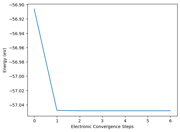
The calculation seems to be converged after the first electronic step with only minimal changes afterwards. But this impression is caused by the misleading representation of the data. If we subtract the full converged energy at the last electronic steps eng_lst[-1] from all other energies and take the absolute of this difference np.abs() then we can plot is on a semi-logarithmic scale. This highlights the logarithmic convergence of the electronic structure, nearly linear with the number of steps in the semi-logarithmic plot.

plt.plot(np.abs(eng_lst-eng_lst[-1]))
plt.xlabel("Electronic Convergence Steps")
plt.ylabel("$\Delta$ Energy (eV)")
plt.yscale("log")

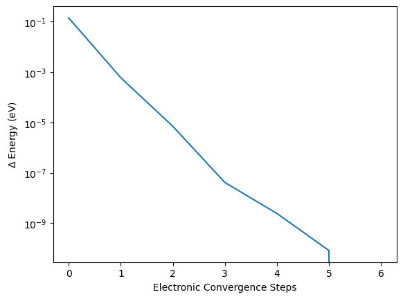
This example demonstrates that determening if a calculation is converged or not always depends on the convergence goal. A convergence of \(10^{-3}\) is already achived at the second electronic step while a convergence of \(10^{-7}\) in this case requires three electronic steps and so on.

Job Management

In the background pyiron uses an Structured Query Language (SQL) database to keep track of the currently running and completed calculation. This has the advantage that old calculation can be reloaded using the load() function of the Project object. Still it can also lead to confusion in the beginning when users try to update the input parameter of an existing calculation. The easiest way is to delete all calculation in a given Project using the remove_jobs() function as demonstrated in the beginning. Alternatively the job object can be reloaded and removed individually by calling the remove() function on the job object. Or to compare multiple calculation the user can simply choose a job_name different from "spx". To get an overview or all job objects in a given project pyiron provides the job_table() function of the Project object.

pr.job_table()

	id	status	chemicalformula	job	subjob	projectpath	project	timestart	timestop	totalcputime	computer	hamilton	hamversion	parentid	masterid
0	1	finished	Al	spx	/spx	None	/home/jovyan/dft/sphinx/	2024-09-03 16:04:14.729280	2024-09-03 16:04:16.997263	2.0	pyiron@jupyter-pyiron-2dsusmet-5fthermodynamics-2dxhwp6iwl#1	Sphinx	3.1	None	None

Conclusion

While for bulk structures electronic convergence is quickly achieved, for more complex chemical structures, surfaces or defects electronic convergence can be much more challenging. So it is important to carefully check the electronic convergence for every calculation.